
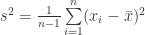
Proof of Unbiasness of Sample Variance Estimator
(As I received some remarks about the unnecessary length of this proof, I provide shorter version here)
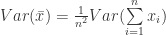
In different application of statistics or econometrics but also in many other examples it is necessary to estimate the variance of a sample. The estimator of the variance, see equation (1) is normally common knowledge and most people simple apply it without any further concern. The question which arose for me was why do we actually divide by n-1 and not simply by n? In the following lines we are going to see the proof that the sample variance estimator is indeed unbiased.


(1)
First step of the proof
(2)

(3)

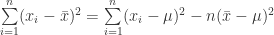
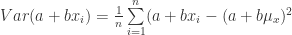
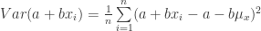
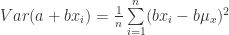
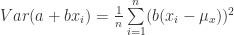
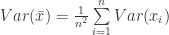
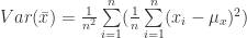
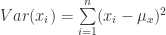
(4)
![(x_i-\bar x)^2 = [(x_i - \mu) + (\mu - \bar x)]^2](https://s0.wp.com/latex.php?latex=%28x_i-%5Cbar+x%29%5E2+%3D+%5B%28x_i+-+%5Cmu%29+%2B+%28%5Cmu+-+%5Cbar+x%29%5D%5E2&bg=ffffff&fg=2b2b2b&s=0&c=20201002)
(5)

(6)

(7)

(8)

(9)

(10)

(11)

(12) 


(13)

(14)

(15)

(16)

(17)

which can be done as it does not change anything at the result
(18)
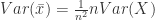
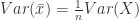
Second step of the proof
(19)

(21)
(22)

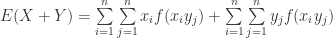
(23)
![E(S^2)=\frac{1}{n}[E(\sum\limits_{i=1}^n (x_i - \mu)^2)-n E(\bar x-\mu )^2]](https://s0.wp.com/latex.php?latex=E%28S%5E2%29%3D%5Cfrac%7B1%7D%7Bn%7D%5BE%28%5Csum%5Climits_%7Bi%3D1%7D%5En+%28x_i+-+%5Cmu%29%5E2%29-n+E%28%5Cbar+x-%5Cmu+%29%5E2%5D&bg=ffffff&fg=2b2b2b&s=0&c=20201002)
Third step of the proof
(24)

(25)
(26)

(27)


(28)

Applying this on our original function:
(29)

(30)

(31)
(32)

(33)

(34)

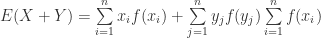
Plugging (34) into (23) gives us:
(35)
![E(S^2)=\frac{1}{n-1}[nVar(x_i)-nE(\bar x-\mu )^2]](https://s0.wp.com/latex.php?latex=E%28S%5E2%29%3D%5Cfrac%7B1%7D%7Bn-1%7D%5BnVar%28x_i%29-nE%28%5Cbar+x-%5Cmu+%29%5E2%5D&bg=ffffff&fg=2b2b2b&s=0&c=20201002)
Notice also that:
(36)
and that:
(37)

(38)

(39)

using (38) and (39) in (37) we get:
(40)
(41)
(42)
(43)
(44)
(45)

(46)

(47)

knowing (40)-(47) let us return to (36) and we see that:
(48)
(49)

(50)
(51)
(52)
just looking at the last part of (51) were we have 
(53)
(54)
now the 

(55)
![Var(X+Y)=E[(X+Y)-(\mu_x+\mu_y)]^2](https://s0.wp.com/latex.php?latex=Var%28X%2BY%29%3DE%5B%28X%2BY%29-%28%5Cmu_x%2B%5Cmu_y%29%5D%5E2&bg=ffffff&fg=2b2b2b&s=0&c=20201002)
(56)
![Var(X+Y)=E[(X-\mu_x)+(Y-\mu_y)]^2](https://s0.wp.com/latex.php?latex=Var%28X%2BY%29%3DE%5B%28X-%5Cmu_x%29%2B%28Y-%5Cmu_y%29%5D%5E2&bg=ffffff&fg=2b2b2b&s=0&c=20201002)
(57)
![Var(X+Y)=E[(X-\mu_x)^2+(Y-\mu_y)^2+2(X-\mu_x)(Y-\mu_y)]](https://s0.wp.com/latex.php?latex=Var%28X%2BY%29%3DE%5B%28X-%5Cmu_x%29%5E2%2B%28Y-%5Cmu_y%29%5E2%2B2%28X-%5Cmu_x%29%28Y-%5Cmu_y%29%5D&bg=ffffff&fg=2b2b2b&s=0&c=20201002)
(58)
![Var(X+Y)=Var(X)+Var(Y)+2(X-\mu_x)(Y-\mu_y)]](https://s0.wp.com/latex.php?latex=Var%28X%2BY%29%3DVar%28X%29%2BVar%28Y%29%2B2%28X-%5Cmu_x%29%28Y-%5Cmu_y%29%5D&bg=ffffff&fg=2b2b2b&s=0&c=20201002)
the term 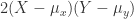
(59)

and playing around with it brings us to the following:
(60)

(61)
(62)
(63)

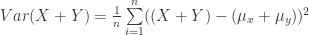
now we have everything to finalize the proof. Return to equation (23)
(64)
![E(S^2)=\frac{1}{n-1}[E(\sum\limits_{i=1}^n(x_i - \mu)^2)-nE(\bar x-\mu )^2]](https://s0.wp.com/latex.php?latex=E%28S%5E2%29%3D%5Cfrac%7B1%7D%7Bn-1%7D%5BE%28%5Csum%5Climits_%7Bi%3D1%7D%5En%28x_i+-+%5Cmu%29%5E2%29-nE%28%5Cbar+x-%5Cmu+%29%5E2%5D&bg=ffffff&fg=2b2b2b&s=0&c=20201002)
and we see that we have:
(65)
![E(S^2)=\frac{1}{n-1}[E(\sum\limits_{i=1}^n Var(x_i))-n\frac{1}{n}Var(X)]](https://s0.wp.com/latex.php?latex=E%28S%5E2%29%3D%5Cfrac%7B1%7D%7Bn-1%7D%5BE%28%5Csum%5Climits_%7Bi%3D1%7D%5En+Var%28x_i%29%29-n%5Cfrac%7B1%7D%7Bn%7DVar%28X%29%5D&bg=ffffff&fg=2b2b2b&s=0&c=20201002)
(66)
![E(S^2)=\frac{1}{n-1}[E(\sum\limits_{i=1}^n \delta^2)-n\frac{1}{n}\delta^2]](https://s0.wp.com/latex.php?latex=E%28S%5E2%29%3D%5Cfrac%7B1%7D%7Bn-1%7D%5BE%28%5Csum%5Climits_%7Bi%3D1%7D%5En+%5Cdelta%5E2%29-n%5Cfrac%7B1%7D%7Bn%7D%5Cdelta%5E2%5D&bg=ffffff&fg=2b2b2b&s=0&c=20201002)
(67)
![E(S^2)=\frac{1}{n-1}[n\delta^2-n\frac{1}{n}\delta^2]](https://s0.wp.com/latex.php?latex=E%28S%5E2%29%3D%5Cfrac%7B1%7D%7Bn-1%7D%5Bn%5Cdelta%5E2-n%5Cfrac%7B1%7D%7Bn%7D%5Cdelta%5E2%5D&bg=ffffff&fg=2b2b2b&s=0&c=20201002)
(68)
![E(S^2)=\frac{1}{n-1}[n\delta^2-\delta^2]](https://s0.wp.com/latex.php?latex=E%28S%5E2%29%3D%5Cfrac%7B1%7D%7Bn-1%7D%5Bn%5Cdelta%5E2-%5Cdelta%5E2%5D&bg=ffffff&fg=2b2b2b&s=0&c=20201002)
so we are able to factorize and we end up with:
(69)
![E(S^2)=\frac{1}{n-1}[\delta^2(n-1)]](https://s0.wp.com/latex.php?latex=E%28S%5E2%29%3D%5Cfrac%7B1%7D%7Bn-1%7D%5B%5Cdelta%5E2%28n-1%29%5D&bg=ffffff&fg=2b2b2b&s=0&c=20201002)
which cancels out and it follows that
(70)

Sometimes I may have jumped over some steps and it could be that they are not as clear for everyone as they are for me, so in the case it is not possible to follow my reasoning just leave a comment and I will try to describe it better.
As most comments and remarks are not about missing steps, but demand a more compact version of the proof, I felt obliged to provide one here.

At last someone who does NOT say “It can be easily shown that…”
In your step (1) you use n as if it is both a constant (the size of the sample) and also the variable used in the sum (ranging from 1 to N, which is undefined but I guess is the population size). Shouldn’t the variable in the sum be i, and shouldn’t you be summing from i=1 to i=n? This makes it difficult to follow the rest of your argument, as I cannot tell in some steps whether you are referring to the sample or to the population.
You are right, I’ve never noticed the mistake. It should clearly be i=1 and not n=1. And you are also right when saying that N is not defined, but as you said it is the sample size. I will add it to the definition of variables.
However, you should still be able to follow the argument, if there any further misunderstandings, please let me know.
it’s very interesting
Thank you!
please how do we show the proving of V( y bar subscript st) = summation W square subscript K x S square x ( 1- f subscript n) / n subscript k …..please I need ur assistant
Unfortunately I do not really understand your question. Is your formula taken from the proof outlined above? Do you want to prove that the estimator for the sample variance is unbiased? Or do you want to prove something else and are asking me to help you with that proof? In any case, I need some more information 🙂
I am very glad with this proven .how can we calculate for estimate of average size
and whats the formula. including some example thank you
I am happy you like it 🙂 But I am sorry that I still do not really understand what you are asking for.
please can you enlighten me on how to solve linear equation and linear but not homogenous case 2 in mathematical method
please how can I prove …v(Y bar ) = S square /n(1-f)
and
S subscript = S /root n x square root of N-n /N-1
and
S square = summation (y subscript – Y bar )square / N-1
I am getting really confused here 🙂 are you asking for a proof of
I like it….
please help me to check this sampling techniques
an investigator want to know the adequacy of working condition of the employees of a plastic production factory whose total working population is 5000. if the junior staff is 4 times the intermediate staff working population and the senior staff constitute 15% of the working population .if further ,male constitute 75% ,50% and 80% of junior , intermediate and senior staff respectively of the working population .draw a stratified sample sizes in a table ( taking cognizance of the sex and cadres ).
I am confused about it please help me out thanx
please am sorry for the inconvenience ..how can I prove v(Y estimate)
Gud day sir, thanks alot for the write-up because it clears some of my confusion but i am stil having problem with 2(x-u_x)+(y-u_y), how it becomes zero. Pls explan to me more.
Hello! The expression is zero as X and Y are independent and the covariance of two independent variable is zero. Does this answer you question?
Regards!
Pls sir, i need more explanation how 2(x-u_x) + (y-u_y) becomes zero while deriving?
See the answer above 🙂
Yes!, thanks alot sir.
You are welcome!
Please I ‘d like an orientation about the proof of the estimate of sample mean variance for cluster design with subsampling (two stages) with probability proportional to the size in the first step and without replacement, and simple random sample in the second step also without replacement. .
Thanks a lot for your help.
Thank you for you comment. The proof I provided in this post is very general. However, your question refers to a very specific case to which I do not know the answer. Nevertheless, I saw that Peter Egger and Filip Tarlea recently published an article in Economic Letters called “Multi-way clustering estimation of standard errors in gravity models”, this might be a good place to start.
Thank you for your prompt answer. I will read that article. Janio
You are welcome! Let me whether it was useful or not.
Thanks a lot for this proof. All the other ones I found skipped a bunch of steps and I had no idea what was going on. Econometrics is very difficult for me–more so when teachers skip a bunch of steps. This post saved me some serious frustration. Thanks!
I’m glad it helped!
Please Proofe The Biased Estimator Of Sample Variance.
What do exactly do you mean by prove the biased estimator of the sample variance? Do you mean the bias that occurs in case you divide by n instead of n-1?
it would be better if you break it into several Lemmas
for example, first proving the identities for Linear Combinations of Expected Value, and Variance, and then using the result of the Lemma, in the main proof
you made it more cumbersome that it needed to be
Hi, thanks again for your comments. I really appreciate your in-depth remarks. While it is certainly true that one can re-write the proof differently and less cumbersome, I wonder if the benefit of brining in lemmas outweighs its costs. In my eyes, lemmas would probably hamper the quick comprehension of the proof. This way the proof seems simple. I like things simple. Cheers, ad.
pls how do we solve real statistic using excel analysis
Hey Abbas, welcome back! What do you mean by solving real statistics? About excel, I think Excel has a data analysis extension. If I were to use Excel that is probably the place I would start looking. However, use R! It free and a very good statistical software. I could write a tutorial, if you tell me what exactly it is that you need.
good day sir.
can u kindly give me the procedure to analyze experimental design using SPSS
Sorry mate. I do not speak SPSS.
Eq. (36) contains an error. There the index i is not summed over.
You are right. I fixed it. Much appreciated.
I think it should be clarified that over which population is E(S^2) being calculated. Is x_i (for each i=0,…,n) being regarded as a separate random variable? If so, the population would be all permutations of size n from the population on which X is defined. I am confused here. Are N and n separate values?
Hey! Thank you for your comment! Indeed, it was not very clean the way I specified X, n and N. I revised the post and tried to improve the notation. Now, X is a random variables, is one observation of variable X. Overall, we have 1 to n observations. I hope this makes is clearer.
Best, ad
I have a problem understanding what is meant by 1/i=1 in equation (22) and how it disappears when plugging (34) into (23) [equation 35]. I feel like that’s an essential part of the proof that I just can’t get my head around. I’ve never seen that notation used in fractions.
Hi Rui, thanks for your comment. Clearly, this i a typo. It should be 1/n-1 rather than 1/i=1. I corrected post. Thanks for pointing it out, I hope that the proof is much clearer now. Best, ad