Log-Linearizing

What exactly is happening when we linearize a model? Well, the answer is simple, we basically approximate non-linear equations with linear once. In context of macroeconomics we may have models which are non-linear. Thus in order to solve them there is need to put them in a linear form. In the following we are going to see how to log-linearizing a model by the means of a (very) simple example.

First of all it is important to remember that a linear approximation is only valid in the close neighborhood of the point from which we linearize. Consequently it is important, when linearizing a model to declare the steady state relation prior the linearization process. In our example the steady state is defined by the variables (c,k,n,z), where c represents consume, k stands for capital, n brings in labor and z the total-factor-productivity.

Knowing the steady state, linearizing the model basically boils down to a Taylor series expansion around the steady state. Suppose we have

(1) $(g(x_{t})=f(y_{t}))$

then we can linear approximate this expression around (x,y) through

(2) $g(x)+g^{'}(x)(x_{t}-x)=f(y)+f^{'}(y)(y_{t}-y)$

And since we are in the steady state $g(x_{t})=f(y_{t})$ implies that $g(x)=f(y)$ as the statement has to be true for any point in time and consequently constants drop out and we end up with

(3) $g^{'}(x)(x_{t}-x)=f^{'} (y)(y_{t}-y)$

Note that this equation is linear in $x_{t}-x$ and $y_{t}-y$ . Now you see that initially in (1) we had something non-linear, but after approximating constants cancel out and we end up with a linear form. It has to be clear that we have something linear in the deviation from out steady state, so it should be clear why the approximation hold only in the immediate neighborhood of the steady state.

Until now we were just talking about the linearization process and not about the logarithmic part. We know from above that in the end we want to end up with something like $g(log(x))=f(log(y))$ , now in order to get there after taking logarithm we have to start from another point: $g(e^{(log(x_{t}))})=f(e^{(log(y_{t})))}$ , approximating this equation around $(log(x),log(y))$ gives us:

(4) $g^{'}(x)x(log(x_t))-log(x))=f^{'}(y)y(log(y_t))-log(y))$

Where in following we will use $log(x_t)-log(x)=(\tilde x_t)$ , which can be interpreted as the percentage deviation of the steady state. Fortunately we do not explicitly have to apply a Taylor series expansion, which could be referred to as the Bruce Force method.

The more elegant method which allows us to circumvent the Taylor series approach is that we approximate

(5) $(\tilde x_{t} )= x e^{(\tilde x_{t} )} \approx x(1+\tilde x_{t} )$

(6) $(\tilde x_{t}) \approx x(1+\tilde x_{t})$

Knowing that $(\tilde x_{t} )$ can be approximated with $x(1+\tilde x_{t})$ , the whole linearization process follows an easy recipe:

1) Replace any variable as $(\tilde x_{t} )$ with $(\tilde x_{t} ) =xe^{(\tilde x_{t}) }$

2) Multiply everything out and simplify as much as possible

3) Approximate $xe^{(\tilde x_t)}\approx x(1+\tilde x_{t})$

Note that $(\tilde x_{t} )*(\tilde y_{t} )\approx 0$ and consequently cancels out.

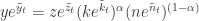
For a deeper understanding of what we are actually going, we are now applying the theoretical description from above on the following equation (7)

(7) $y_t=z_t k_t^{\alpha} n_t^{1-\alpha}$

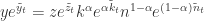
1) Replace any variable with $\tilde x_{t}$ as $\tilde x_{t} = xe^{(\tilde x_t )}$

(8) $ye^{\tilde y_{t}}=ze^{\tilde z_{t}} (ke^{\tilde k_t})^{\alpha} (ne^{\tilde n_t})^{(1-\alpha)}$

2) Multiply everything out and simplify as much as possible gives us

(9) $ye^{\tilde y_{t}}=ze^{\tilde z_{t}} k^{\alpha} e^{\alpha \tilde k_t} n^{1-\alpha} e^{(1-\alpha)\tilde n_t}$

From (7) follows that the steady state relation is $y=zk^\alpha n^{(1-\alpha)}$ , consequently it cancels out in (9) and we end up with

(10) $e^{\tilde y_t}=e^{\tilde z_t} e^{\alpha \tilde k_t} e^{(1- \alpha)\tilde n_t}$

3) Approximate $xe^{x_t}\approx x(1+\tilde x_t)$ or $e^{x_t}\approx(1+\tilde x_t)$

(11) $1+\tilde y_t \approx (1+\tilde z_t)(1+\alpha \tilde k_t)(1+(1-\alpha)\tilde n_t)$

(12) $1+\tilde y_t \approx(1+\tilde z_t+\alpha \tilde k_t+\tilde z_t\alpha \tilde k_t)(1+(1-\alpha) \tilde n_t )$

(13) $1+\tilde y_t \approx(1+\tilde z_t+\alpha \tilde k_t)(1+(1-\alpha) \tilde n_t )$

(14) $1+\tilde y_t \approx(1+\tilde z_t+\alpha \tilde k_t+\tilde n_t+\tilde z_t\tilde n_t+\alpha \tilde k_t\tilde n_t+(1-\alpha) \tilde n_t + (1-\alpha) \tilde z_t\tilde n_t+(1-\alpha)\alpha \tilde k_t\tilde n_t)$

(15) $1+\tilde y_t \approx (1+\tilde z_t+\alpha\tilde k_t+(1-\alpha) \tilde n_t)$

(16) $\tilde y_t \approx \tilde z_t+\alpha\tilde k_t+(1-\alpha) \tilde n_t$

Where (16) is the approximation for (7).

Economic Theory Blog

Log-Linearizing

Leave a Reply Cancel reply

“In God we trust; all others must bring data.” W. Edwards Deming

Share this:

Leave a Reply Cancel reply

“In God we trust; all others must bring data.” W. Edwards Deming