The usual way of interpreting the coefficient of determination 


Another way of interpreting the coefficient of determination 

In the following we are going to see how to derive the coefficient of determination

The usual way of interpreting the coefficient of determination
Another way of interpreting the coefficient of determination

![Cov[\hat{y},e]=0](https://s0.wp.com/latex.php?latex=Cov%5B%5Chat%7By%7D%2Ce%5D%3D0+&bg=ffffff&fg=2b2b2b&s=0&c=20201002)
![Cov[x,(y+Z)]=Cov(x,y)+Cov(x,Z)](https://s0.wp.com/latex.php?latex=Cov%5Bx%2C%28y%2BZ%29%5D%3DCov%28x%2Cy%29%2BCov%28x%2CZ%29&bg=ffffff&fg=2b2b2b&s=0&c=20201002)


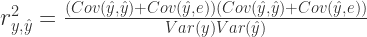
![r_{y,\hat{y}}=\frac{Cov(y,\hat{y})}{\sqrt[2]{Var(y)Var(\hat{y}) }}](https://s0.wp.com/latex.php?latex=r_%7By%2C%5Chat%7By%7D%7D%3D%5Cfrac%7BCov%28y%2C%5Chat%7By%7D%29%7D%7B%5Csqrt%5B2%5D%7BVar%28y%29Var%28%5Chat%7By%7D%29+%7D%7D&bg=ffffff&fg=2b2b2b&s=0&c=20201002)
In the following we are going to see how to derive the coefficient of determination
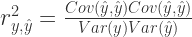
![r^{2}_{y,\hat{y}}=\left(\frac{Cov(y,\hat{y})}{\sqrt[2]{Var(y)Var(\hat{y}) }}\right)^{2}](https://s0.wp.com/latex.php?latex=r%5E%7B2%7D_%7By%2C%5Chat%7By%7D%7D%3D%5Cleft%28%5Cfrac%7BCov%28y%2C%5Chat%7By%7D%29%7D%7B%5Csqrt%5B2%5D%7BVar%28y%29Var%28%5Chat%7By%7D%29+%7D%7D%5Cright%29%5E%7B2%7D&bg=ffffff&fg=2b2b2b&s=2&c=20201002)
![r^{2}_{y,\hat{y}}=\frac{Cov(y,\hat{y})}{\sqrt[2]{Var(y)Var(\hat{y}) }} \frac{Cov(y,\hat{y})}{\sqrt[2]{Var(y)Var(\hat{y}) }}](https://s0.wp.com/latex.php?latex=r%5E%7B2%7D_%7By%2C%5Chat%7By%7D%7D%3D%5Cfrac%7BCov%28y%2C%5Chat%7By%7D%29%7D%7B%5Csqrt%5B2%5D%7BVar%28y%29Var%28%5Chat%7By%7D%29+%7D%7D+%5Cfrac%7BCov%28y%2C%5Chat%7By%7D%29%7D%7B%5Csqrt%5B2%5D%7BVar%28y%29Var%28%5Chat%7By%7D%29+%7D%7D&bg=ffffff&fg=2b2b2b&s=2&c=20201002)


Thank you for this!
You are very welcome!
Hi Isidore: Do you know if the relation between the correlation coefficient R and r holds for the regression model with ma(1) errors ? empirically I seem to find that it doesn’t hold. but I wanted to make sure that my code didn’t have a bug. thanks for any wisdom and your blog.
Hi Mark! That is actually a very good question which unfortunately I cannot answer out of the box. However, once I have some time I will look into it. So far my feeling is that the second of the five bullet points (listed in the post), i.e. the covariance between the fitted values and the error term being equal to zero, is most likely violated. Generally I think if you are able to show that all five bullet points hold for a ma(1) process, the relationship between r2 and the correlation coefficient should hold as well.
Let me know if you find an answer to the question.
Cheers!
Thanks Isidore: What you pointf out is equivalent to the sums of squares decomposition relation , SSETOT = SSREG + SSE, being true. So I think I should look for info on when that decomposition holds in general. cov(y hat, e ) not being zero makes it not true so your pont is a good one. Thanks and I’ll let you know if I find anything out about it.
How did you get from covar(x,y) to covar(y’,y)?
Thank you for your comment. I am sorry, but I cannot really help you as I do not understand to which equation you are referring to. If you could be more specific I might be able to help.
Regards
Hello, can you tell me what you do between the pictures, i don’t quite understand it
Hello, what do you mean by pictures?
Thanks a lot for this. Maybe, one possible small typo is: ESS/TSS should be RSS/TSS? This is true as the mean of y^hat is equal to the mean of y, as the mean of e_i is zero.
Thank you for your comment. EES stands for “Explained Sum of Squares”, whereas RSS stands for the “Residual Sum of Squares”. Hence ESS/TSS is correct.
Best, ad
o sorry, I guess I was wrong as ESS is as “Explained SS” .
Exactly, ESS stands for “Explained Sum of Squares”. Best ad
Very interesting content – thanks!
For some reason I fail to see the intuition behind the second last line. Why can var(y^) be said to be equal to ESS?
Does this have to do with the assumptions behind the y^ line? Coulnd’t there be variance in this regression line which doesn’t contribute to explaining the variance in y?
I hope my question makes sense
Hi, this is a very good question. I was to short on this point. I will adjust the post such that it becomes more clear. The short answer is, plug in the variance equation two times and cancels out. What remains are the sum of squared residuals.
Thanks for this comment.
ad
Thank you. I think there is some missing squares on the second last line, no? var(y) = sum((yi-mean(y))^2)/n, and the same thing for the estimates.
Thank you for you comment. You are right, of course! I adjusted the post. Cheers, ad